How a camera's sharpness is actually measured. The page begins with what MTF and SFR
mean and why the ISO 12233 method uses a slanted edge; sets out the synthetic chart the
measurements come from and the assumptions the method rests on; follows the analysis
pipeline step by step, including where the resolution comes from and why the
conventional tilt is conventional; asks whether the pipeline recovers an answer it was
never given; and ends with what five common image-quality conditions — contrast, noise,
vignetting, distortion and gamma — do to the result.
Every section states its conclusion plainly, including the ones that do not
flatter the tool.
A camera does not have a resolution. It has a response, and that response
depends on how fine the detail is. A lens that renders a 10-cycle-per-degree pattern
faithfully may render a 40-cycle pattern as uniform grey. "How sharp is it" is therefore
not a number until you say at what spatial frequency.
MTF — the property of the system
The Modulation Transfer Function is contrast out divided by contrast in,
as a function of spatial frequency. It is a curve, not a score.
ISO 12233's measurable: the edge response normalised to unity at zero
frequency. The estimated MTF is the SFR divided frequency-by-frequency by the input
edge's own modulation.
SFR is a system measurement — it does not separate lens from sensor
Physically the chain is a product: light passes the lens, then lands on silicon that
integrates it over a finite pixel and lets charge spread to neighbours. So the system
response is approximately
The aperture term is the sinc of the pixel's finite size — a pixel is an averaging
box, and averaging blurs. The diffusion term is charge wandering into neighbouring
pixels, which is why the effect is called crosstalk.
But the standard measures the product, never the parts. A slanted-edge
SFR is a number for the whole camera. Nothing in this repository — or in ISO 12233 —
decomposes it into lens and sensor contributions. Treating a measured SFR as a lens
MTF is the most common misreading of this measurement, and it is wrong.
One further caution: aperture and diffusion are not independently separable
by simple multiplication. The real sensor MTF is somewhat higher than the product,
and the discrepancy grows with crosstalk — so the convenient model above is
optimistic rather than exact.
Where ISO 12233 comes in
ISO 12233 is the standard that defines how to measure this from a
single photographic capture. It specifies a high-contrast edge tilted a few degrees
from the pixel grid, and the analysis chain that turns that edge into an SFR curve.
This repository implements that method in full, over a synthetic chart whose correct
answer is known in advance — which is what makes the validation section a validation
rather than a comparison against another black box.
Notation and units
Two frequency units appear on this page and they are not interchangeable. Everything
internal is cycles per pixel; lp/mm appears only where a sensor's physical pitch is known.
Quantity
Unit
Range here
Reference points
Frequency axis
cycles / pixel
0 – 0.5
Nyquist is 0.5 by definition
mtf50
cycles / pixel
0 – 0.5
cannot exceed Nyquist
ny4_sfr
MTF, unitless
0 – 1
Ny/4 = 0.125 cy/px
ny2_sfr
MTF, unitless
0 – 1
Ny/2 = 0.25 cy/px
Edge tilt
degrees from axis
2 – 15
shipped default 5
Blur
pixels (σ, Gaussian)
0 – 3
0 is an ideal edge
mtf50_lpmm
line pairs / mm
sensor-dependent
$\text{mtf50}\times 1000 / \text{pitch}_{\mu m}$
The last row is why the 0.5 ceiling matters. On a 2.2 µm sensor, 0.5 cy/px is 227 lp/mm —
so a system sharper than Nyquist is not measurable here, only unresolvable.
That distinction is the subject of the validation section.
Why the edge has to be slanted
A sensor answers one question per pixel: how much light landed here. A vertical edge
lands on the same sub-pixel position in every row — so every row measures the same
phase, and the edge profile is known only at one sample per pixel. You cannot resolve
detail finer than that, and you cannot even represent it.
Tilt the edge and the arithmetic changes. Each row crosses the boundary at a different
fraction of a pixel, so the rows collectively sample the transition at many different
sub-pixel positions. The tilt is not a convenience — it is the measurement.
The phase advance
Moving down one pixel row shifts where the edge crosses it by tan θ
pixels. Consecutive rows therefore land on different phases.
$$\Delta_{\text{phase}} = \tan\theta \ \ \text{pixels per row}$$
The phase span
Over an edge L rows long, the phases sweep this far. It must exceed one
pixel for the sampling to interleave at all.
The equivalent sampling interval is the pixel pitch divided by this —
at the conventional 5° over a 32-row edge, roughly 11× finer than the sensor
could otherwise manage.
$$\text{oversampling} = \frac{1}{\tan\theta}$$
Two failure modes bound the usable angle, and they pull in opposite directions. Too
shallow and the phase coverage becomes non-uniform — angles whose slope is a
simple rational number (0°, tan⁻¹(1/4) ≈ 14.04°, tan⁻¹(1/2) ≈ 26.57°, 45°) repeat a small
set of phases and leave ESF bins empty. Too steep and the binning corrections the
method relies on grow, biasing the result. ISO 12233 prescribes roughly 2–10° and gives
surprisingly little justification; the section on the tilt sweep measures where this
implementation's optimum actually falls.
Method and assumptions
Every number on this page comes from a chart this repository generates. Because the
generator knows exactly what it applied, the correct answer is known in advance — that
is the whole basis for the validation.
The test chart
Grayscale, single channel. No colour filter array, no demosaic, no
colour processing. A real camera's SFR is measured on luminance for exactly this
reason: it keeps the measurement independent of colour reconstruction.
8-bit. 256 levels. The generator supports 8, 10, 12, 14 and 16.
Dark level 38, light level 191 — a 5:1 contrast ratio. Dark is
pinned at 15% of full scale; light is dark × ratio, clamped at 85%. The clamp is why
the contrast sweep stops at ratio ≈ 5.6: beyond that the chart is byte-identical.
3 × 3 grid of slanted squares, 88 px across on a 266 px pitch in an
800 × 800 field — 36 measurable edges.
8× supersampled and box-downsampled, so the ideal edge is
anti-aliased rather than staircased. This is the one blur present even at
“zero” blur, and the validation section has to account for it.
Assumptions the method rests on
These are not caveats bolted on at the end — they are the conditions under which the
numbers mean anything. The image-quality metrics section tests each of them.
The edge is straight. The analysis fits one angle and one
projection axis. A curved edge has no single angle, so the projection smears.
The blur is constant across the region of interest. The profile
measured in one part of the ROI is assumed to hold for all of it.
The signal is linear in light. Contrast ratios and MTF only compose
as ratios on a linear scale. ISO 12233's procedure linearises via the OECF first;
this implementation does not, and the gamma results show what that costs.
You know where the edge is. The measurement is only as good as the
registration under it.
What can be varied
Knob
What it does
Range used here
resolution
Field size in pixels
800 × 800
slant_angle
Edge tilt; sets the phase coverage
2 – 15°
contrast_ratio
Light/dark ratio of the squares
1.2 – 5.6
blur_type, blur_sigma
Gaussian blur, in pixels
σ = 0 – 3
defocus_radius
Pillbox (disk) blur alternative
not used on this page
snr_db
Signal-to-noise ratio
15 – 60 dB
vignetting_strength
Corner darkening
0 – 0.35
distortion_type, distortion_k
Barrel / pincushion warping
k = 0 – 0.25
gamma
Tone curve applied to the chart
1.0 – 2.7
bit_depth
Quantisation
8
square_size, square_pitch
Square geometry
auto (11% of field)
The pipeline, step by step
Thirty-six edges, four per square. Each step below gives the operation, the mathematics,
and what the code actually does — the step that matters most is the fourth.
detect_squares()
Find the chart. Otsu threshold separates squares from background;
contours give candidate blobs; a rotated bounding box filters them by area and aspect
ratio. Squares are then grouped into rows by clustering the gaps in their
y coordinates, so the code adapts to any grid layout rather than assuming 3×3.
When the chart is synthetic the known geometry is passed in instead and this step is
skipped entirely.
_refine_edge_position()
Snap to the true edge. A bounding box locates an edge only to
within a pixel or so. This searches ±10 px along the edge normal for the position of
maximum gradient — cheap, and it removes most registration error. Everything
downstream inherits this accuracy or its absence.
_extract_edge_roi()
Cut a region shaped for the method. Long along the edge
(0.5 × the square) and shallow across it (0.4 ×, minimum 20 px). The asymmetry is
deliberate: many independent cross-sections are useful, but only the pixels near the
transition carry information, and a deeper ROI would only add flat regions that
contribute nothing but noise to the derivative.
compute_esf()
Project, then bin. The step that turns a photograph into a
measurement. Detailed below.
$$p = y - x\tan\theta \quad\text{(horizontal edge)}$$
$$p = x - y\tan\theta \quad\text{(vertical edge)}$$
compute_lsf()
Differentiate, then taper. The Line Spread Function is the
derivative of the ESF — the edge's step response differentiated gives the impulse
response, which is what the transform needs.
The differentiated profile is then multiplied by a Tukey window (α = 0.25). The
window is at full height where the LSF has signal and tapers only where the LSF is
already near zero, which suppresses spectral leakage without attenuating the peak.
compute_sfr()
Transform and normalise. An FFT with 2× zero padding for finer
frequency sampling, magnitude normalised to the DC term, restricted to
$0 \le f \le 0.5$ cy/px.
From that curve: mtf50 by linear interpolation of the 0.5 crossing,
and the values at Ny/4 and Ny/2 read off directly.
Project and bin, in detail
This is where the resolution comes from, so it is worth following slowly.
1 · Every pixel gets a coordinate
Each pixel in the ROI is assigned a single number: its position along the edge
normal, $p$. Because the edge is tilted, two pixels in the same column but different
rows receive different values of $p$ — that is the entire trick. In a
32-row ROI at 5°, the $p$ values advance by 0.0875 px per row.
2 · The rows become cross-sections
Read a single row and you have a one-dimensional cut through the edge, sampled
once per pixel — coarse and phase-dependent. But every row is a cut through
the same edge at a slightly different offset. Projecting them all onto the
common $p$ axis stacks those cuts on top of one another, and what was 1 sample per
pixel becomes many samples per pixel.
3 · Bin at ¼ pixel
The projected samples are collected into bins 0.25 px wide, and
each bin reports the mean of the pixels that landed in it. The bin width is the
reconstruction grid: the ESF is being rebuilt on a grid four times finer than the
sensor's own sample spacing. That factor of four is the oversampling, and it
is what allows the FFT in the next step to report frequencies up to 0.5 cy/px
instead of stopping at the edge of what the pixel grid could represent.
At 5° with a 32-row ROI the phases sweep 2.7 px, so roughly eleven distinct
positions fall inside each 0.25 px bin — enough that the mean is a real average
rather than a single sample in disguise.
4 · Normalise and orient
Bins with no samples are filled by interpolation. The profile is then scaled to
[0, 1] and forced ascending, so a dark-to-light edge and a light-to-dark edge produce
the same LSF sign. Polarity is detected from the ROI's own halves, not assumed.
Why ¼ pixel? It is the ISO 12233 convention — a fixed reconstruction
grid, independent of the tilt. The tilt controls something different: how many distinct
phases actually populate those bins. A steep edge starves the bins; a shallow one
over-samples a narrow phase range and risks rational-slope degeneracy. The
tilt sweep measures where the optimum falls for this
implementation, and it lands on the conventional value.
So why 5°? Swept
Error against the 5° reference for seven angles from 2° to 15°,
each the mean of 36 edges at 1 px blur. Effective oversampling falls from 28.6× at 2°
to 3.7× at 15°.
The conventional value is the measured optimum here
Error is at its minimum near 4–5° and climbs monotonically to 2.96%
at 15°, tracking the collapse in phase coverage. The penalty at 2° is small —
0.22% — and much weaker than the high-angle effect.
That asymmetry matches the physics: the high-angle penalty comes from the binning and
derivative corrections, which grow steadily with tilt, while the low-angle penalty only
bites when the phase coverage becomes degenerate. The 5° default is not a
knife-edge optimum — anything from about 3° to 7° would measure equivalently
well here — but it sits comfortably inside the safe region, and it is what ISO 12233
prescribes.
Watching it happen
Every image below is produced by running this repository's own code.
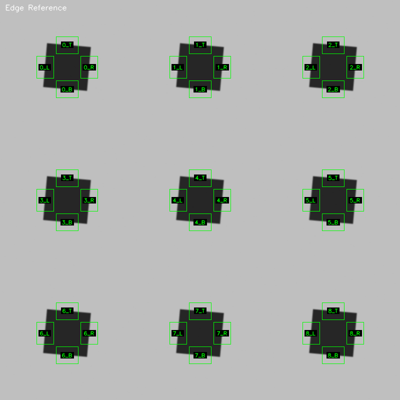
Thirty-six edges, indexed {square}_{T|B|L|R}.
Squares run 0–8 left-to-right, top-to-bottom. The labels are the handles every number
on this page is reported against, which is why a per-edge CSV is more useful than a
summary: it lets you see which edges disagree.One edge, magnified. The boundary crosses pixel rows at a
different phase in each row — that is the entire mechanism. A perfectly axis-aligned
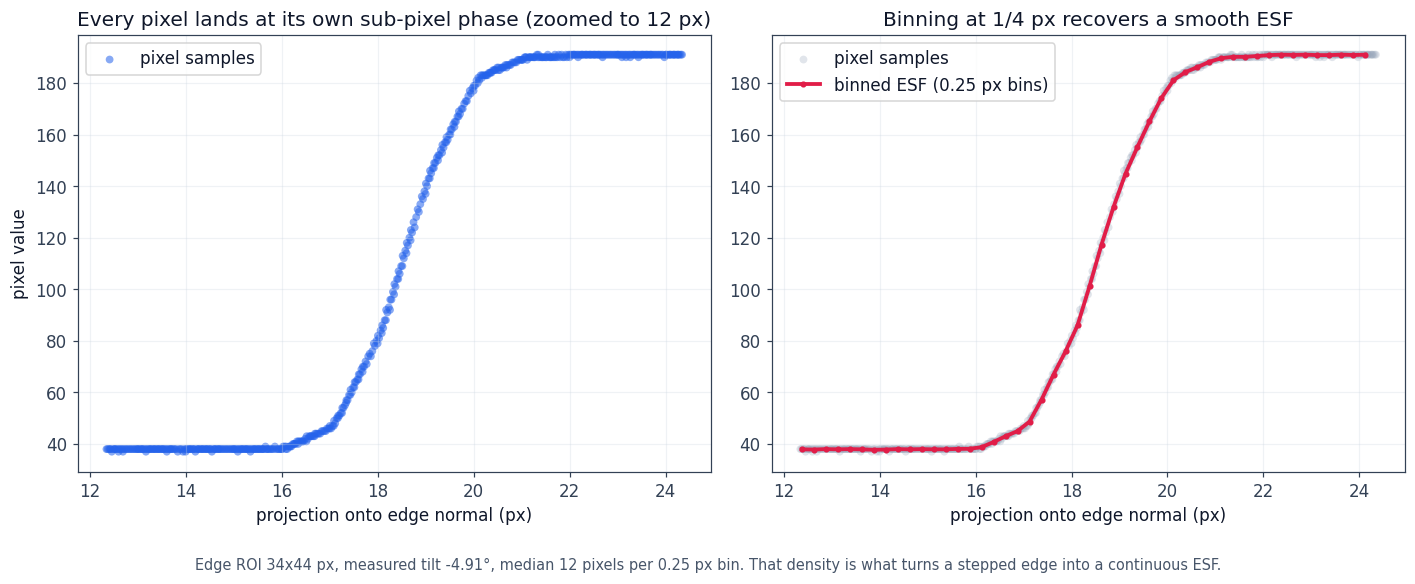
edge would sample the same phase forever and the ESF would be a staircase.Where the sub-pixel information comes from. Left, each pixel
lands at its own fractional position along the edge normal — no two rows share a phase.
Right, averaging into ¼-pixel bins recovers a continuous ESF from a sensor that can only
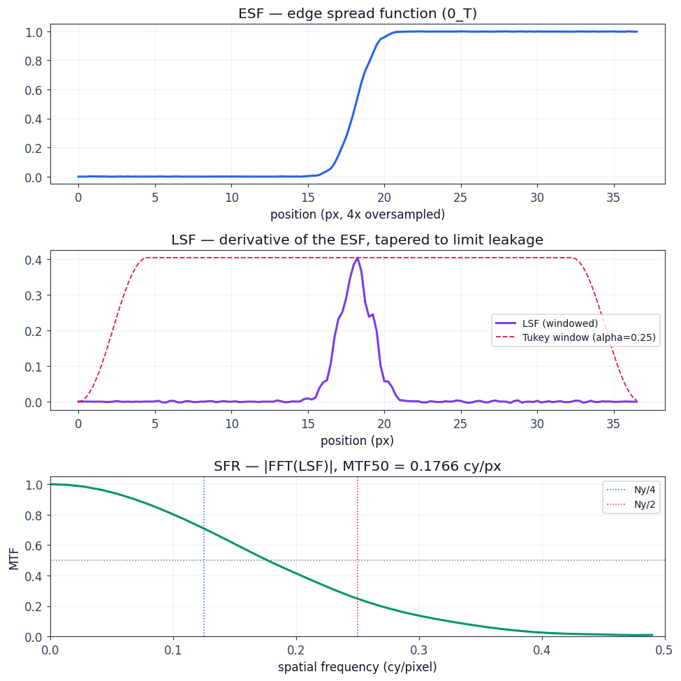
report integers. The tilt is not a convenience; it is the measurement.The chain, end to end. Note the middle panel: the Tukey
window is at full height exactly where the LSF has signal and tapers only where the LSF
is already zero. That is why this window rather than a Hamming — it suppresses spectral
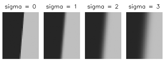
leakage without paying for it in the region you care about.What the blur sweep actually varies. The same edge at
σ = 0, 1, 2 and 3 px. Every number in the validation section is read off charts like
these — the transition widening is the only thing that changes, which is what makes the
comparison against theory meaningful.
Try the tilt yourself
This is step 4 of the pipeline, running live. The left panel is the chart at the pixel
level — the boundary is drawn in red and the blue ticks in the margin mark where each
row crosses it. The right panel is the ESF those same pixels produce when you project
and bin them. Drag the angle and watch the two panels stay in step.
The readout reports phase step — how far the boundary advances per row —
and phase span — how much of a pixel it sweeps in total. Both are
measured against the 0.25 px bin: once the step exceeds the bin width, samples can skip
bins entirely, and the readout says so.
The chart, at the pixel level. Every row
crosses the boundary at a different fraction of a pixel.
The ESF those pixels produce. Fewer
distinct phases means a coarser reconstruction.
Validation
The generator knows what blur it applied, so the correct MTF50 is known in advance.
Seven blur levels, thirty-six edges each. The question is not whether the curve looks
plausible — it is whether the measurement recovers a number it was never given.
What theory predicts
Two factors form the prediction: the pixel's finite size, which
averages light over its area (a sinc), and the applied Gaussian blur. A third,
INHERENT_BLUR_SIGMA = 0.2, accounts for the chart's own anti-aliasing —
the edge is not a mathematical step, so it carries a little blur of its own.
Measured MTF50 against theory Validated above σ = 1 px
Where the validator can score, measurement and theory agree to
between 0.01% and 0.22%. The marked point at σ = 0 is not a comparison at all.
Above σ = 1 px: the pipeline recovers the answer
The worst error across the whole measurable band is 0.22%, at
σ = 1.5 px it is 0.01%. Nothing in the measurement was given the
correct value — it is recovered from the image alone. This is the validation.
sigma measured theory error verdict
0.0 0.4570 0.5000* -- *clamped, not a prediction
0.5 0.3512 0.3056 14.95% scored; model least accurate here
1.0 0.1771 0.1767 0.22% scored
1.5 0.1216 0.1216 0.01% scored
2.0 0.0921 0.0923 0.16% scored
2.5 0.0742 0.0742 0.10% scored
3.0 0.0620 0.0620 0.09% scored
Below σ ≈ 0.1 px there is nothing to compare against
Pixel aperture alone crosses MTF = 0.5 at 0.603 cy/px, and with the chart's own blur
included the true MTF50 at σ = 0 is 0.5155 — both beyond the 0.5 the
frequency axis can represent. The validator searches only to 0.5, so it returns that
limit instead of a crossing, and the 8.59% gap there is the validator running out of
range rather than the analyzer being wrong.
The region is narrow: the true MTF50 drops back inside Nyquist at σ ≈ 0.1 px, so a
sweep in 0.5 px steps catches it at exactly one point. That is why the chart above shows
the theory curves touching the dashed line rather than a shaded band.
How image quality metrics impact SFR measurement
Five conditions, each tested the same way: what it does to the image, what that does to
the measurement, the number, and the mechanism behind it. Two of them barely matter, one
sets a hard floor, and two are measurable artifacts that have nothing to do with
sharpness.
Summary. MTF50 is normalised, so anything that scales the
whole image — contrast, gain, vignetting — largely cancels. What does not cancel is
anything that changes the shape of the edge (gamma), the scale of the
image (distortion), or the noise on top of it (SNR). That single distinction
predicts every result below.
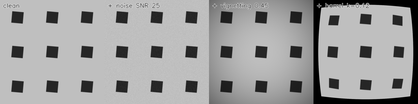
The five conditions, four of them visible. Same chart,
four captures: clean, noise, vignetting, distortion. Gamma is the fifth and is not
visible by eye — which is precisely why it needs measuring rather than inspecting.
1 · Contrast
TL;DR Contrast does not change MTF50 — the metric is normalised, so gain cancels exactly. It only sets a floor: below about 2:1 no edge is measurable at all.
Physically: the luminance difference between the square and its
background. To the measurement: because MTF is normalised to unity at
zero frequency, contrast cancels out of the ratio — so contrast should not change MTF50
at all, only how reliably it can be measured.
The number: contrast sets a floor, not a trend
From ratio 2 upward MTF50 is flat at ≈ 0.177 cy/px across a 2.8×
contrast range — exactly as a normalised metric should behave.
Below that it collapses as a measurement, not as a value: at ratio 1.2 and
1.5, 0 of 36 edges pass the quality gate. The edge gradient falls
below the minimum the detector requires, so the pipeline is measuring edges it has
already judged unfit.
Mechanism: a low-contrast edge carries less signal above the noise, so
the gradient used to locate and bin the edge becomes unreliable. Note also the ceiling:
the generator clamps the light level at 85% of full scale, so ratios above ≈ 5.6
produce a byte-identical chart. The usable contrast window is narrow — roughly
2:1 to 5.6:1.
2 · Signal-to-noise ratio
TL;DR Noise leaves the MTF50 value almost untouched and destroys its reliability: the spread across edges falls about 100× from 15 dB to 60 dB, while the mean barely moves.
Physically: how much of the signal survives above the noise floor.
To the measurement: noise does not shift MTF50 so much as make it
unstable — the error is in the spread across edges, not the mean.
The number: precision scales with SNR, over more than two orders of magnitude
The spread falls by a factor of ~100 from 15 dB to 60 dB, while the
mean MTF50 stays near 0.177 throughout. Noise degrades the confidence in the
measurement, not its value — which is why a single-edge MTF number from a noisy image
should not be trusted even when it looks reasonable.
Mechanism: the ESF is an average over the pixels in each bin. Noise
averages down as √N, so more binning or more signal both tighten it — but at low SNR
the edge position itself becomes ambiguous, which biases as well as scatters it.
3 · Vignetting
TL;DR Almost harmless — 2.4% centre to corner — because MTF is a ratio and vignetting is a gain. The measurement’s real limit is edge-to-edge spread at 12.4%, five times larger.
Physically: illumination and aperture fall off toward the corners, so
the same scene produces less signal at the edge of the field.
To the measurement: this is a gain change, and MTF is a ratio — so it
should largely cancel.
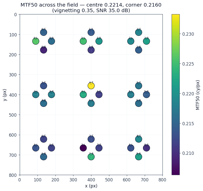
The same measurement as a map. Each point is one edge at its
physical position. The colour varies substantially between edges of the same square —
the spread is local, not radial.
The number: 2.4% centre-to-corner, and 12.4% between neighbours
effect magnitude
centre -> corner falloff 2.42%
edge-to-edge spread 12.43%
Strong vignetting (0.35) moves MTF50 by only 2.42% from centre to
corner — because the ESF is normalised to [0,1] and the MTF to its own DC term, and both
divisions remove exactly what vignetting changes. Measuring MTF through a vignetted
field is legitimate because the metric is contrast-normalised.
The far more useful number is the second one. Edge-to-edge spread is five
times the field trend, which is the quantitative reason real MTF testing
averages over many edges and reports a distribution rather than one number.
Mechanism: the residual 2.4% is consistent with the noise term —
less light at the corners means a noisier ESF. That is the expected mechanism, not a
measured one: no vignetting-off control was run.
4 · Distortion
TL;DR Distortion moves the chart, so the region of interest must follow it or you are measuring registration error. Even correctly registered, the local magnification change shifts what “cycles per pixel” means.
Physically: the lens maps the field with a position-dependent
magnification, bending straight lines and moving the chart.
To the measurement: the region of interest must follow that map. If it
does not, the analysis window sits on the wrong part of the edge and you are measuring
registration error rather than optics.
Three things follow, and only the first is obvious
The ROI must track the distortion map. Placing regions of interest at
the pre-distortion positions produced a non-monotonic mess; inverting the map and
placing them where the squares actually landed produced a clean, monotonic result.
Registration is not a refinement here — it is the difference between a measurement and
noise.
Automatic detection fails outright, at any non-zero level. Even
k = 0.02 returns zero edges. The remap fills the frame border with black — the same
value as the dark squares — so thresholding turns that border into foreground and
contour retrieval returns one box covering the whole image, which fails the area
filter. Given known positions, all 36 edges are still measured.
Even correctly registered, cycles per pixel changes meaning. Barrel
distortion demagnifies the periphery, so the same edge is drawn across fewer pixels and
its detail lands at higher cycles per pixel. MTF50 rises from 0.177 to 0.203
across this sweep — a 14% apparent improvement in sharpness from a defect that cannot
improve sharpness. The metric is reporting local scale, not local resolution.
5 · Gamma
TL;DR The one metric that genuinely breaks the
measurement. With a near-black edge against a bright one the bias reaches
−13%, because the signal is analysed without the linearisation
ISO 12233 prescribes.
Physically: a tone curve applied to the signal, as every camera does to
fit a wide luminance range into a limited code space. To the measurement:
MTF is defined on a linear signal. Unlike contrast, which cancels, a tone curve
changes the shape of the edge and does not cancel.
Method note. This is the one metric measured on a constructed edge
rather than a generated chart: the generator pins dark at 15% of full scale and clamps
light at 85%, capping any chart it makes at 5.67:1. The gamma model
(apply_gamma) and the measurement (analyze_edge) are still this
repository's own — only the input image is built directly.
This is a named deviation from ISO 12233
The ISO 12233 slanted-edge procedure includes an OECF linearisation
step — the opto-electronic conversion function is measured and the edge linearised
before it is differentiated. This implementation omits that step and
measures the encoded signal directly, which is the situation of analysing sRGB output
without decoding it. Everything below follows from that.
Bias against the dark edge's level Up to −13%
Light level fixed at 85% of full scale; dark level swept from
0.39% to 50%. The green marker is where the generator's own chart sits — the mild
end, and the only place a chart-based sweep could have looked.
The number: it scales with how dark the dark edge is
dark % of full scale contrast ratio bias at gamma 2.2
1 0.39% 217:1 -13.30%
2 0.78% 108:1 -11.36%
8 3.14% 27:1 -6.97%
16 6.27% 14:1 -4.75%
32 12.55% 7:1 -2.75%
64 25.10% 3:1 -1.18%
128 50.20% 2:1 -0.23%
That is a 58× span. For reference, the same gamma applied to
the generator's own chart — a 5:1 ratio — costs 1.97%, which
is the figure a chart-based sweep reports as the whole story. At the regime that
matters in practice, a dark object against a bright background, the error is an order
of magnitude larger.
Mechanism. Encoding applies $v^{1/\gamma}$, whose slope
$(1/\gamma)\,v^{1/\gamma-1}$ diverges as $v \to 0$. Near zero the curve is both
steepest and most curved, so a dark edge sits exactly where the encoding distorts the
edge profile most.
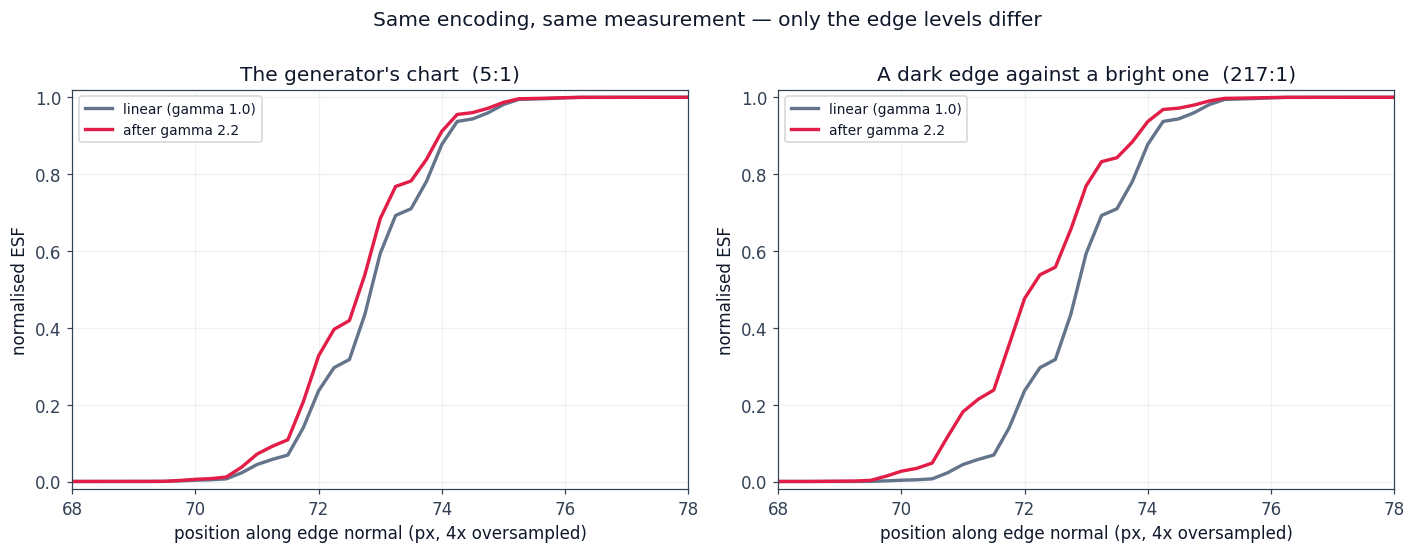
The distortion itself, same gamma in both panels. On the
left the chart's own 5:1 edge barely moves. On the right, a near-black edge against the
same bright background is pulled visibly earlier and steeper — which is the whole
effect. Only the edge levels differ; the encoding and the measurement are identical.
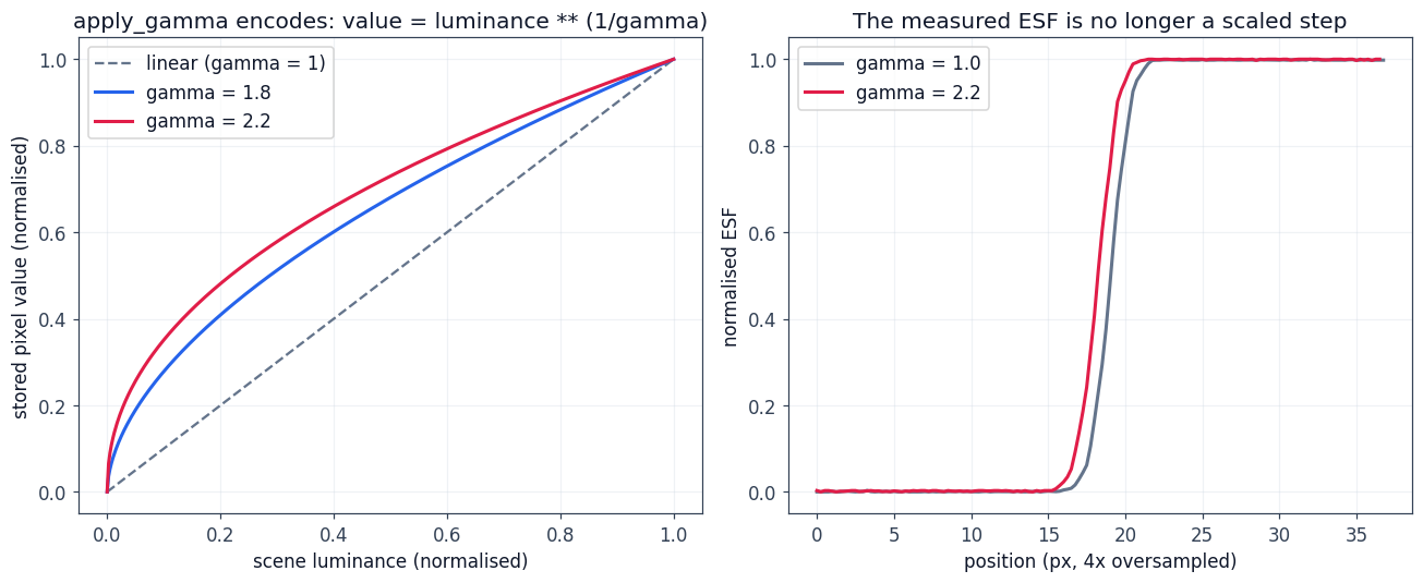
Why the dark end is where it bites. The curves climb
steeply out of the origin and flatten toward the top — so an edge near black is
remapped hard while an edge near white is barely touched. That asymmetry skews the
LSF and moves MTF50.
It is the ratio that matters, and most of the damage is done by gamma 1.8
A power law is scale-invariant, so the distortion depends on the ratio
between the two edge levels, not on where they sit in absolute terms. Holding the ratio
fixed while dropping the dark level 20× gives an identical bias every time —
−0.22% at dark levels of 24, 48, 96, 192 and 384 alike. At a fixed full scale the
two coincide, since a darker object is a higher ratio, but the mechanism is the
ratio.
Most of the damage arrives by gamma 1.8 and the curve flattens after that. So the
practical question is not which gamma value a camera uses — it is whether the pipeline
linearises at all.
Using it
Install
git clone https://github.com/pengzhao-ai/SFR_Slanted.git
cd SFR_Slanted
python -m venv .venv && source .venv/bin/activate
pip install -r requirements.txt
pip install -e .          # optional: enables the sfr-analyzer entry point
Generate a chart, then measure it
# 3x3 slanted-square chart, 1 px of Gaussian blur, with its config saved
python -m sfr_analyzer generate --resolution 400 400 --angle 5 \
    --blur-sigma 1.0 --output test.png --save-config

# measure all 36 edges; writes overlays, SFR curves and results.csv
python -m sfr_analyzer analyze --input test.png --pixel-pitch 2.2 --output results/

# compare the measurement against theory for the parameters that made it
python -m sfr_analyzer validate --input test.png --config test.json --output report.txt
API
from sfr_analyzer import SyntheticImageGenerator, SFRAnalyzer, ValidationModule

gen = SyntheticImageGenerator(resolution=(800, 800), slant_angle=5.0,
                              blur_type="gaussian", blur_sigma=1.0)
gen.generate()

an = SFRAnalyzer(pixel_pitch_um=2.2)
an.set_image(gen.generate())
results = an.analyze(gen.get_square_info())   # dict keyed by "0_T" ... "8_R"
an.export_csv("results.csv")

v = ValidationModule(pixel_pitch_um=2.2, blur_sigma=1.0, blur_type="gaussian")
print(v.validate(results).summary())
Passing gen.get_square_info() uses known geometry and skips detection
entirely — faster and more accurate, but only available when you control the chart.
Omit it to exercise the automatic path, which is what the distortion finding above
concerns.