Optical degradation

Question

Can the toolkit classify the dominant optical degradation in an image, and does the manifest adapter plus the reporting layer generalize beyond CIFAR-10?

This is a framework and diagnostics showcase. The images are 32×32 CIFAR-10 base images with synthetic degradations, so it is not a production image-quality benchmark.

Classes

Label	Optical analogue	Implementation
clean	no dominant degradation	unchanged
defocus	defocused PSF	Gaussian blur
motion_blur	motion during exposure	oriented line kernel
chromatic_aberration	wavelength-dependent magnification	per-channel radial scale
vignetting	off-axis illumination falloff	radial gain mask
sensor_noise	photon and read noise	Gaussian + Poisson
jpeg	compression artifacts	JPEG round-trip

flowchart LR
    Deg["Optical degradation"] --> Clean["clean"]
    Deg --> Blur["defocus / motion_blur"]
    Deg --> Color["chromatic_aberration / vignetting"]
    Deg --> Sensor["sensor_noise / jpeg"]

flowchart LR
    Group["Base image group"] --> Split["Assign split before generation"]
    Split --> Train["train"]
    Split --> Val["validation"]
    Split --> Test["held-out test"]
    Train --> Manifest["manifest.csv + generated images"]
    Val --> Manifest
    Test --> Manifest

Severity is sampled per sample from a configured range and written to the manifest.

Data and split

The generator uses selected CIFAR-10 training images as base images. Each base image is a group; groups are assigned to train/validation/test before any degraded sample is generated. The manifest records:

path,label,split,group,severity

The manifest adapter reads the CSV and the explicit split column. The generator is deterministic for a seed, and the --quick path uses fewer base images.

Model and report

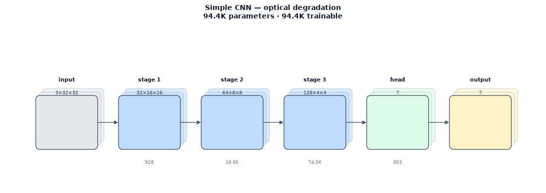
A small simple_cnn with 32/64/128 channels and 94,375 parameters trains through the same trainer, evaluator, and report path as the CIFAR demos. The schematic shows the stage shapes; the report includes the confusion matrix, per-class metrics, calibration, and an error gallery. The useful analysis is which degradations are confused with which.

Result

2,100 generated samples; 420 test samples (60 per class).

Field	Value
Test accuracy	85.71%
Test macro F1	85.57%
Test accuracy 95% CI	82.38–88.81%
Best validation accuracy	82.38% (epoch 16)
Latency	0.70 ms/image

Class	F1	Support
clean	70.18%	60
defocus	92.68%	60
motion_blur	85.00%	60
chromatic_aberration	100.00%	60
vignetting	78.33%	60
sensor_noise	91.80%	60
jpeg	80.99%	60

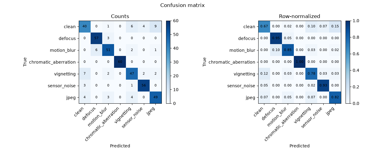
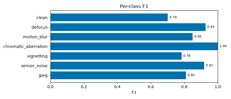
Clean is the hardest class, as expected for subtle degradations at 32×32. Chromatic aberration, defocus, and sensor noise are classified reliably.

• Generator
• Config
• Demo
• Results

What to notice

• A second dataset needs no code changes. Only the adapter and config change.
• Group leakage is checked before generation. No base image appears in two splits.
• The diagnostics are the point. Confusion and calibration are more useful than a single accuracy number.
• The caveat is explicit. 32×32 synthetic degradations are a framework demonstration.

Caveat

Some optical effects are subtle at 32×32. The demo does not claim production image-quality performance; it shows that the data, training, evaluation, and reporting layers generalize to a manifest-based task.